BACI evaluation Baviaanskloof

library(spatialBACI)
library(terra)
#> terra 1.8.86

The Baviaanskloof dataset

We here use a part of the Baviaanskloof dataset used in del Río-Mena et al., 2021, included in the spatialBACI package, to demonstrate a pixel-based before-after-control-impact (BACI) evaluation using the package. The Baviaanskloof dataset contains the sites of large-scale spekboom (Portulacaria afra) revegetation in the semi-arid Baviaanskloof Hartland Bawarea Conservancy, South-Africa. Attributes the vector dataset indicate in which year the revegetation was undertaken by the different restoration organizations active in the area (Commonland, Living Land, Grounded) and whether lifestock grazing exclusion was implemented as a restoration activity. As an example, we here select the sites revegetated in 2012 that were not subject to lifestock grazing exclusion.

data(baviaanskloof)
baviaanskloof <- unwrap(baviaanskloof)

year <- 2012
impact_sites <- baviaanskloof[baviaanskloof$Planting_date==year & baviaanskloof$Lifestock_exclusion==0]
other_sites <- baviaanskloof[baviaanskloof$Planting_date!=year | baviaanskloof$Lifestock_exclusion==1]

plot(baviaanskloof, "Planting_date", xlab="Longitude", ylab="Latitude")
lines(impact_sites, lwd=2)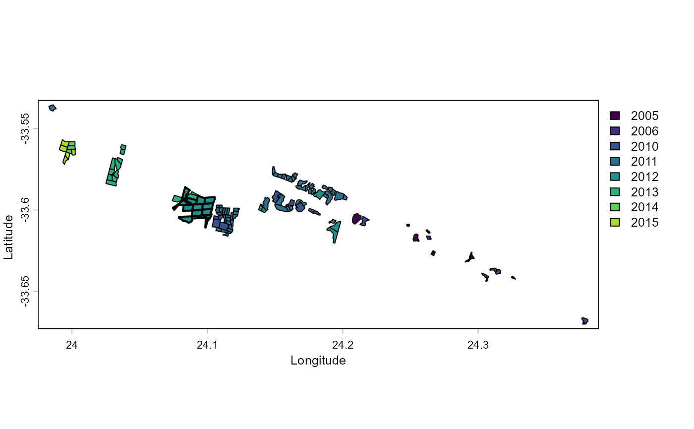

Defining impact and control units

The spatialBACI package requires the user to define the spatial unit at which the analysis will be performed. The options for this are the pixel unit (using raster-based analysis) or the polygon/point unit (using vector-based analysis). The latter can be useful when working with extensive networks of fixed monitoring sites from which the control sites can be expected. One of the advantages of the pixel unit is that it is not required that candidate control sites are predefined. Another advantage is that, depending on the size of impact sites and spatial resolution of the used remotely sensed datasets, information on impact within an impact site can be assessed. For this example we will use pixels as the spatial unit of analysis and reporting.

When using a raster-based analysis, the first choice the user will have to make is the spatial resolution of the pixel units. We here choose a spatial resolution of 60m, since this is a resolution to which several Earth Observation datasets (e.g., Landsat, Sentinel-2) can be aggregated. The next step is to identify the area from which the control pixels for the Before-After-Control-Impact an be selected. The spatialBACI package provides several options for this. The first option is by providing a spatial window around the impact units, the second is providing a polygon identifying the area from which to select the control pixels. The package also provides options to exclude areas from use as control in the BACI analysis. This exclusion can be based on user-provided polygons, or buffer area around the impact sites (e.g., to eliminate the effect of misregistration of impact sites or of positive or negative adjacency effects). All these options to include or exclude candidate control units can be combined based on the user’s terrain knowledge and data availability in the create_control_candidates() function. In this example, we set a window of 5 km around the sites reforested in 2012 (with the control_from_buffer argument) and exclude areas restored in the other years as control pixels (with the control_exclude argument). Finally, we use the argument exclude_impact_buffer to exclude pixels in a buffer of 300 m around the impact sites for selection as control units. The create_control_candidates function also allows us the specify the Coordinate Reference System (trough the crs argument) of the reference raster at which the analysis will be done. This can be useful if, e.g., the user wants to use a national reference system. In our example we don’t provide the crs parameter, in which case the UTM zone of centroid of the impact sites will be used. Setting the round_coords argument to -2 sets the origin of the output SpatRaster to the closest 100 m, and setting the sample_control argument to 0.5 results in a random sampling of 50% of the candidate control pixels, which can be useful to reduce computational load for large study areas.

impact_control_cands <- create_control_candidates(impact_sites,
                                                  resolution=60,
                                                  control_from_buffer=5000,
                                                  control_from_include=NULL,
                                                  control_exclude=other_sites,
                                                  exclude_impact_buffer=300,
                                                  round_coords=-2,
                                                  sample_control=0.5)

plot(impact_control_cands)
lines(project(impact_sites, impact_control_cands))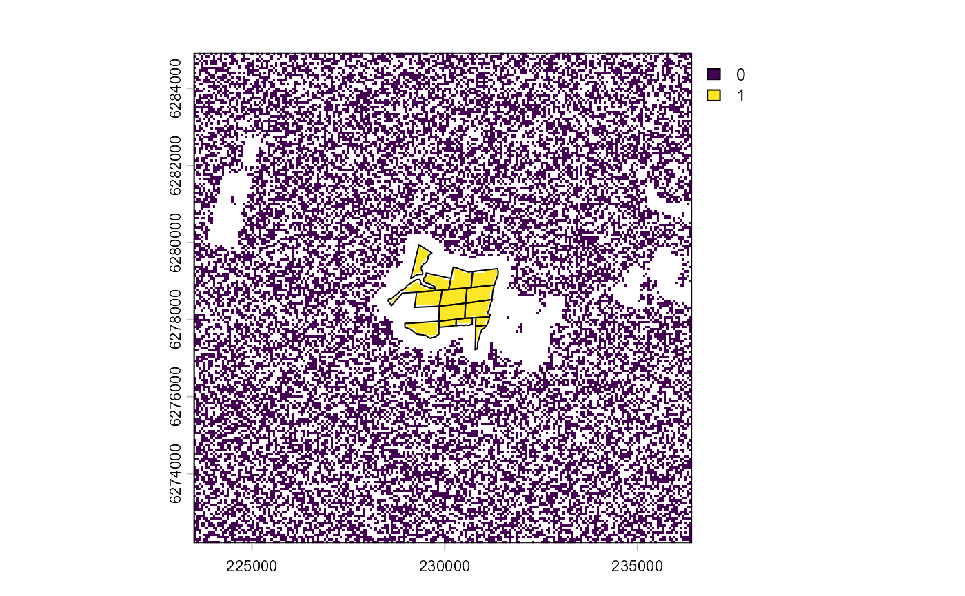

The resulting plot shows the impact units/pixels (1), the candidate control units/pixels (0), and the pixels excluded from analysis in white. Notice that the plot shows UTM coordinates, rather than the geographic coordinates of the Baviaanskloof reference dataset. In general, the spatialBACI package will automatically check the crs of used spatial datasets and reproject when required.

Control-Impact Matching

In impact assessment using control-impact (of before-after-control-impact) schemes, it is crucial that the control units are carefully selected so that their characteristics only differ from those of the impact group by the received “treatment” (in our case a restoration intervention). This is in the spatialBACI package done by specifying a set of covariates to be used in the matching analysis. Ideally, users should include “all covariates likely to impact both the selection to the treatment and the outcome of interest” (Schleicher et al., 2019).

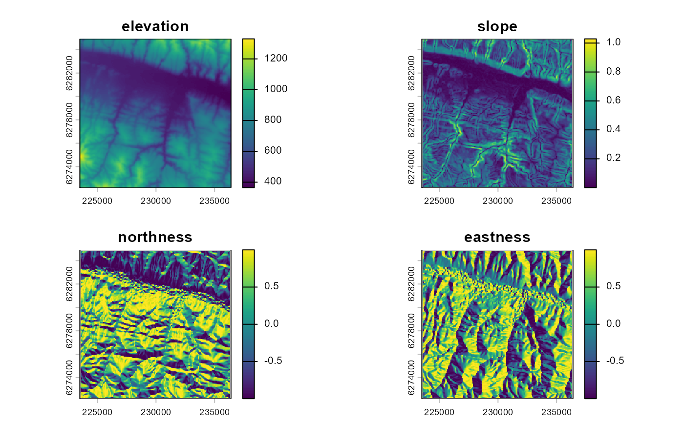
For the Baviaanskloof example, we use a limited number of matching covariates. Because we restricted the search window for control units to a relatively small area around the impact sites, we assume that climatic variation will be small and mostly induced by local topography. Topographic slope and aspect may also determine whether or not a site is selected for revegetation or determine the success of the revegetation intervention. This terrain data can be extracted from the NASA Digital Elevation Model (DEM) based on SRTM data using the dem() function. Unless specified otherwise, the DEM will be obtained from Microsoft’s Planetary Computer. The user can also specify the terrain derivatives to be calculated (by default the slope and the aspect), and whether the aspect should be transformed to “northness” and “eastness” by applying the cosine and sine function on it (default) or not.

dem_matching <- dem(impact_control_cands)
plot(dem_matching)

We also included land cover as a matching covariate. This will ensure that control pixel are selected from the same landcover type (i.e. “rangeland”). Note that in the current implementation of the lulc() function, the 9-class land use land cover layer from Impact Observatory is used. This product is first generated for the year 2017, so we assume no change in land cover change between the intervention year (2012) and 2017. Given that terrain revegetated with spekboom will still be classified as “rangeland” this is not an issue in this example, but it may be a problem for other situations.

landcover_matching <- lulc(impact_control_cands, year=year)
#> Warning in .local(x, year, endpoint, collection, assets, authOpt, ...): Land
#> cover product io-lulc-9-class currently has data 2017-2022. 2017 selected.
plot(landcover_matching)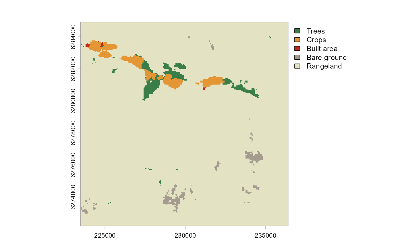

Distance to roads or settlements can explain the anthropogenic pressure on an area. The spatialBACI package therefore includes functions to calculate the distance to the nearest road (osm_distance_roads()) or nearest settlement (osm_distance_places()) based on OpenStreetMap data. For this example, we include the distance to the nearest road of OSM category “track” or higher as an environmental covariate in the matching analysis.

roadsDist_matching <- osm_distance_roads(impact_control_cands, values="track+")
plot(roadsDist_matching)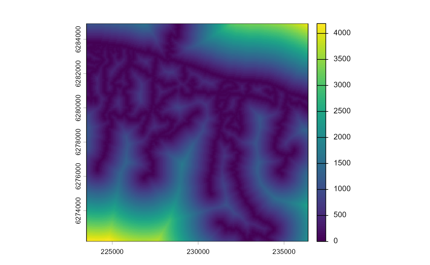

The different matching covariates can be easily collated into a format that can serve as input to the control-impact matching with the collate_matching_layers() function. This function handles the necessary spatial processing of the different spatial input layers, which may have different coordinate systems or spatial resolutions.

matching_input = collate_matching_layers(impact_control_cands, vars_list=list(dem_matching, landcover_matching, roadsDist_matching))

The function test_multicollinearity() plots a correlation matrix of the matching covariates, reports their Variance Inflation Factor (VIF), and allows the user to iteratively identify and remove highly multicollinear covariates. In our example, VIF values for all covariates are low (<5), so we choose to keep all of them in the matching.

matching_input = test_multicollinearity(matching_input)

We then perform the control-impact matching with the matchCI() function using propensity score matching (default method), and select 10 control pixels for each impact pixel (argument ratio) with replacement (argument replace), meaning that a control pixel can be paired with several impact pixels.

matching_output <- matchCI(matching_input, 
                           ratio=10, replace=TRUE)

The function evaluate_matching() performs some standard assessments of the matching output. Under the default parameters, the function generates plots of the covariate distribution, and a Love plot of Standardized Mean Differences for control and impact sites before and after matching. From the output of the matching analysis, we can see that the absolute Standardized Mean Difference after matching is below the threshold of 0.1 for the propensity score distance, only barely above this threshold for a few individual covariates. Based on these outputs we can continue our analysis with the current matching output, as we do here, or reject the matching and attempt matching with different matching parameters or covariates.

evaluate_matching(matching_output) 
#> Balance Measures
#>                           Type Diff.Adj
#> distance              Distance  -0.0000
#> elevation              Contin.   0.0488
#> slope                  Contin.  -0.1147
#> northness              Contin.  -0.0086
#> eastness               Contin.   0.0721
#> landcover_Trees         Binary   0.0000
#> landcover_Crops         Binary   0.0000
#> landcover_Built area    Binary   0.0000
#> landcover_Bare ground   Binary   0.0000
#> landcover_Rangeland     Binary   0.0000
#> dist_roads             Contin.   0.0471
#> 
#> Sample sizes
#>                       Control Treated
#> All                  20436.       691
#> Matched (ESS)         3569.68     691
#> Matched (Unweighted)  4614.       691
#> Unmatched            15822.         0
#> Press <Enter> to continue.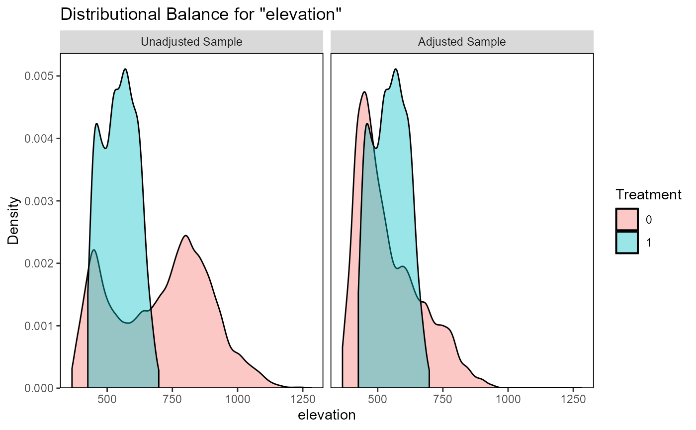

#> Press <Enter> to continue.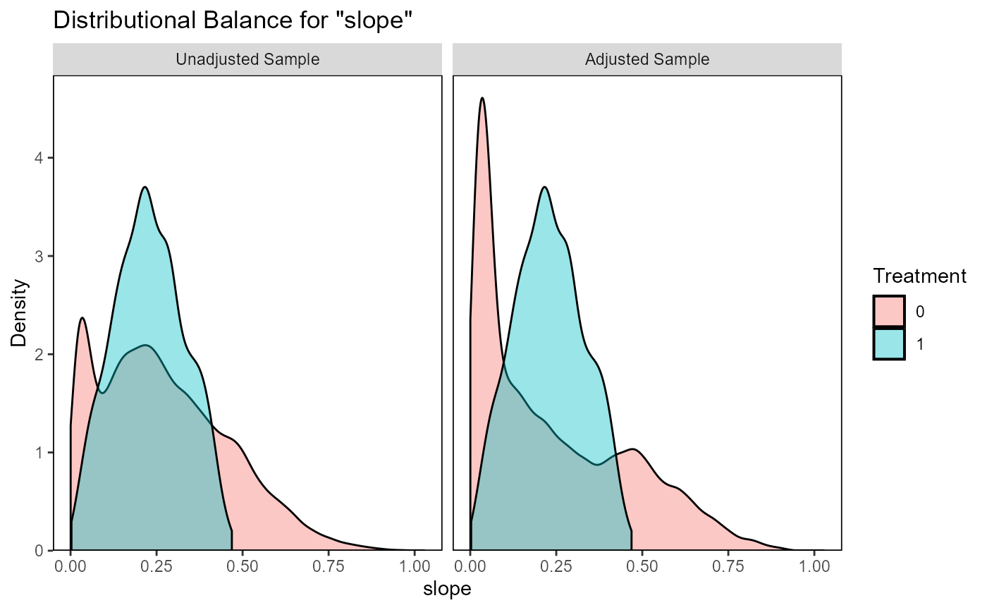

#> Press <Enter> to continue.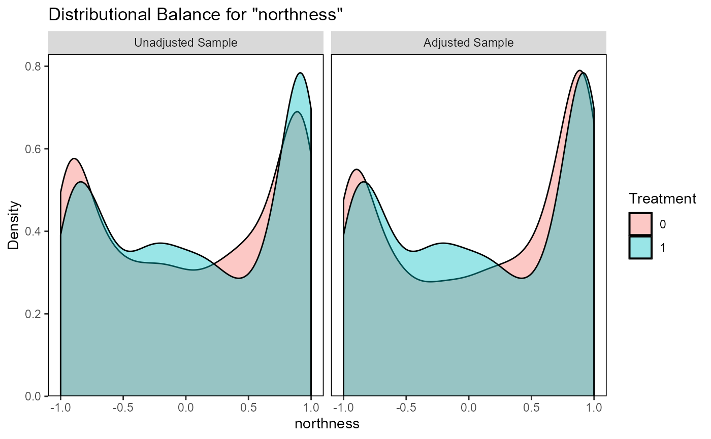

#> Press <Enter> to continue.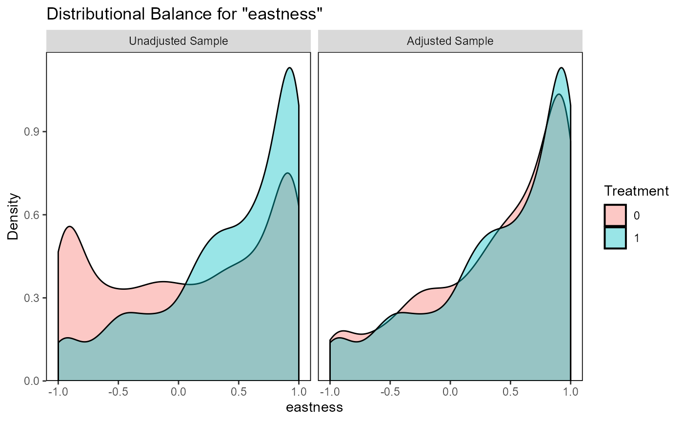

#> Press <Enter> to continue.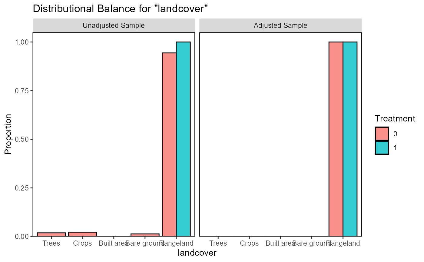

#> Press <Enter> to continue.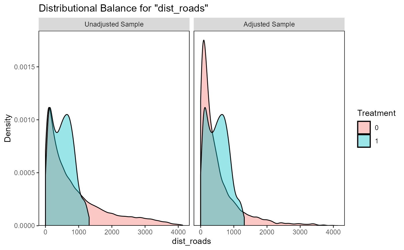

#> Press <Enter> to continue.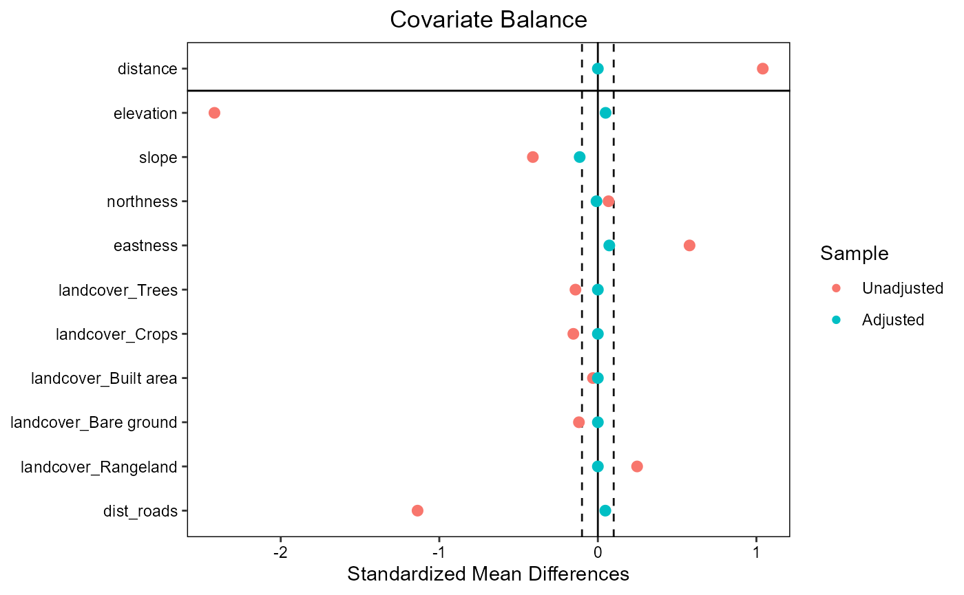

#> Press <Enter> to continue.

Impact assessment

Remotely sensed observables

We here chose Landsat Normalized Difference Vegetation Index (NDVI) as the metric to use in the impact evaluation. NDVI is indicative of vegetation “greenness” and could therefore inform us whether a large scale revegetation effort was successful. The Landsat programme has been running for several decades and is therefore a useful data source for impact evaluation of past interventions. Landsat data are available from several cloud platforms. We here use Microsoft’s Planetary Computer, which allows querying with the SpatioTemporal Asset Catalog (STAC) language.

stac_endpoint <- as.endpoint("PlanetaryComputer")
stac_collection <- as.collection("Landsat", stac_endpoint)

The timeframes over which conservation or restoration impacts are assessed will depend on the application and study site. Assuming we want to evaluate the impact of the Baviaanskloof revegetation from the 5-year periods before and the 5-year after the intervention year, we can first generate yearly NDVI time series for all impact and candidate control pixels:

vi_before <- eo_VI_yearly.stac(impact_control_cands, "NDVI",
                               endpoint=stac_endpoint, collection=stac_collection,
                               years=seq(year-10, year-1, 1),
                               months = 3:5,
                               maxCloud=60)
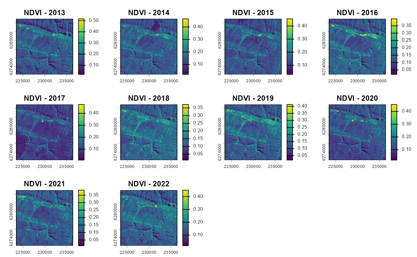
vi_after <- eo_VI_yearly.stac(impact_control_cands, "NDVI",
                              endpoint=stac_endpoint, collection=stac_collection,
                              years=seq(year+1, year+10, 1),
                              months = 3:5,
                              maxCloud=60)

In the above code, we specified that we want to make a pixel-based NDVI composite image for each year, using for each pixel and each year the median value from the images acquired in the months March until May that have a cloud cover below 60%. The function eo_VI_yearly.stac() above generates proxy data cubes, which don’t contain any data but describe the dimension of the object. Data retrieval and calculations are only performed when the data values contained in these objects are needed. Working with data cubes has the advantage that unnecessary calculations are avoided for bands, time steps and/or coordinates that are not used in later steps. This can be extremely useful when dealing with large areas from which only limited data has to be extracted, e.g., sparse monitoring location distributed over a continental-scale area. In such a case you do not want to process data wall-to-wall over the continental scale, but only over these sparse locations. In our Baviaanskloof example, however, we only cover a geographically small area with a relatively dense cover of impact and candidate control units. In such case it can be useful to transform the data cubes to SpatRaster objects (from terra package) with the as.SpatRaster() function. Doing this downloads and processes all data and reads the resulting composite images into memory (or writes them to temporal files).

vi_before <- as.SpatRaster(vi_before)
vi_after <- as.SpatRaster(vi_after)
plot(vi_before, main=paste0("NDVI - ",seq(year-10, year-1, 1)))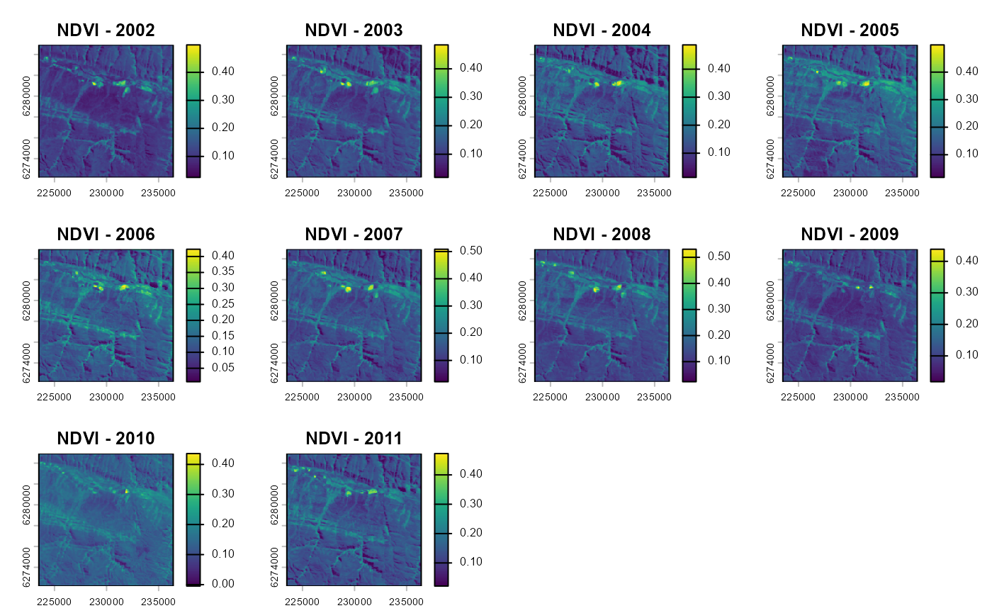

plot(vi_after, main=paste0("NDVI - ",seq(year+1, year+10, 1)))

To transform these time series into simple metrics that can be used in a BACI analysis, we here calculate average value and trend (change in NDVI/year) over the time series before and after intervention with the calc_ts_metric() function. This basic time series analysis is included in the spatialBACI package, but user can easily implement their own analyses, as long as these return raster layers of the evaluation variable of interest before and after intervention.

avgtrend_before <- calc_ts_metrics(vi_before)
avgtrend_after <- calc_ts_metrics(vi_after)

BACI contrast and p-value

To run the BACI analysis, we need to provide the matched control-impact pairs (output of matchCI()) and the raster datasets of the before and after period to the BACI_contrast() function. The BACI analysis will be performed for all layers in the before and after layers, which in our example are both the average and trend over the time series.

baci_results <- BACI_contrast(matching_output, before=avgtrend_before, after=avgtrend_after)

The results of the BACI analysis can be viewed by printing the data.table associated to the output object. The data.table shows, for each impact unit and each evaluation variable, the BACI contrast and p-values. BACI contrast values smaller than zero indicate a positive effect of the revegetation intervention.

head(baci_results$data)
#> Key: <subclass>
#>    subclass  cell treatment contrast.average p_value.average contrast.trend
#>      <fctr> <int>     <num>            <num>           <num>          <num>
#> 1:        1 18158         1     -0.007516017     0.107309678  -5.215998e-06
#> 2:        2 18373         1     -0.007124912     0.001719528  -1.234128e-06
#> 3:        3 18374         1     -0.006553027     0.036084266  -1.076089e-06
#> 4:        4 18375         1     -0.000707540     0.871349236  -3.731212e-06
#> 5:        5 18588         1     -0.002613761     0.677131688  -7.347847e-06
#> 6:        6 18589         1     -0.002799080     0.489423545  -6.619877e-06
#>    p_value.trend
#>            <num>
#> 1:    0.14678868
#> 2:    0.66389019
#> 3:    0.57750778
#> 4:    0.10941389
#> 5:    0.03418171
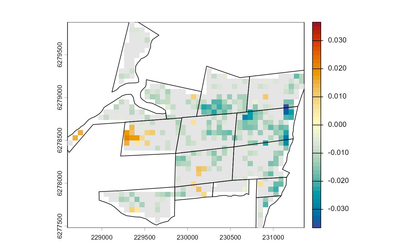
#> 6:    0.02101184

The BACI results can also be plotted on a map, here with non-significant BACI contrast masked out. If desired, the pixel-based results can now be aggregated to different spatial levels, e.g., the revegetation site.